Schrödinger Notes—Molecular Docking

Declaration

This note contains only minimal annotations to the original text, along with corrections to formatting errors. It is intended for educational and communicative purposes only, and all rights remain with the original author.

Introduction

Glide is a Schrödinger module that performs ligand-receptor docking reliably. To run a Glide virtual screen, you need a grid file and a ligand file. The grid file is typically generated from a prepared protein (using Protein Preparation Workflow and Receptor Grid Generation), and the ligand file is processed by LigPrep.

Prepare the Protein Using the Protein Preparation Workflow

This section is based on the article, “Introduction to Structure Preparation and Visualization”¹, and created with the Schrödinger Software Release 2023-4.

Structure files obtained from the PDB, vendors, and other sources often lack necessary information for performing modeling-related tasks. Typically, these files are missing hydrogens, partial charges, side chains, and/or whole loop regions. Proteins in their raw state may also have incorrect bond order assignments and group orientations. To make these structures suitable for modeling tasks, we will use the Protein Preparation Workflow to resolve common structural issues.

1. Start Maestro, then import the protein and include it

• e.g. Go to File > Get PDB to download 1FJS

2. In the Favorites toolbar, click Protein Preparation

• The Protein Preparation Workflow opens

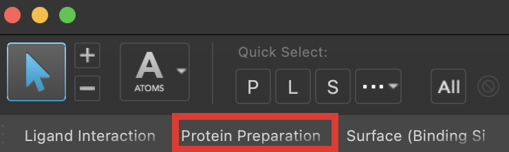
Figure 2-1. The Protein Preparation Workflow in the Favorites toolbar.

3. Switch to Preparation Workflow tab, confirm the Interactive button is off

• When on, the pane will read Protein Preparation Workflow (interactive)

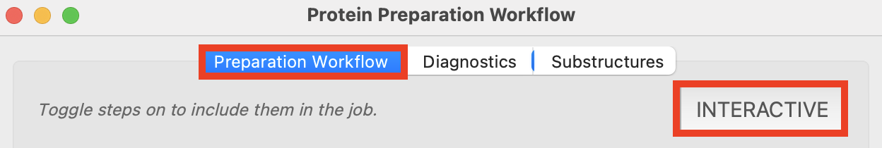
Figure 2-2. The Protein Preparation Workflow in Automatic mode.

Note

Interactive mode can be used for exploring manual options, or to run a single protein in a step-by-step manner. This tutorial will be running an automatic protein preparation.

4. In the Specify Protein section, choose use structures from: Workspace

5. Select Global Settings

• A dropdown opens showing the simulation pH and the PDB pH as well as small molecule options

Note

Simulation pH text box: Enter the pH value to use for the protein's aqueous environment. The default is 7.4, the physiological pH. If the PDB structure has a pH value, and it is different from this value by more than 1 pH unit, a warning is posted, as the processed protein structure could deviate from that in the input structure. In this case you can select Use PDB value instead to use the reported pH.²

6. Select Review Structure

• The substructures tab opens to show Ligands, Metals, Other, Waters, and Chains

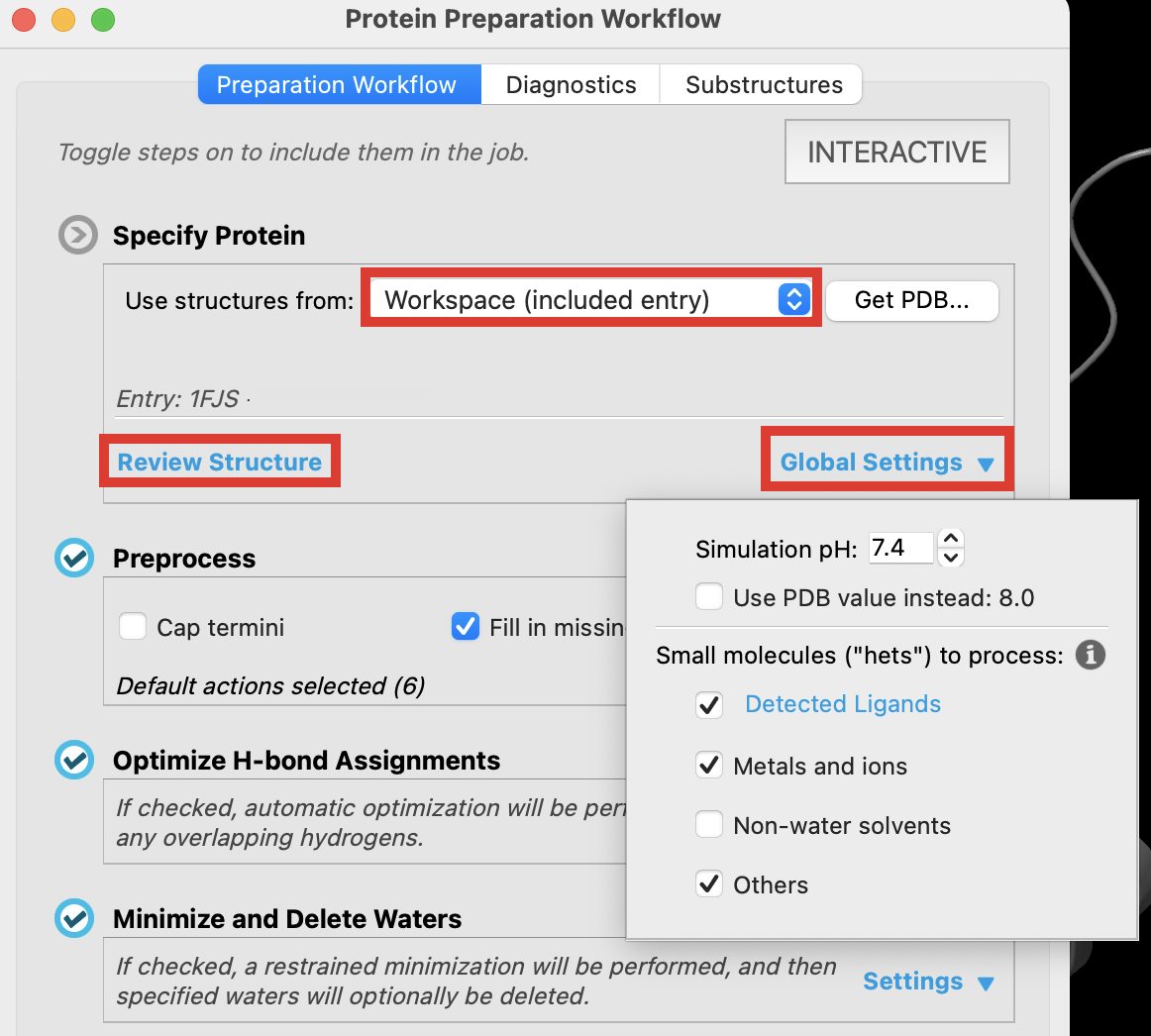
Figure 2-3. Specify the protein from the Workspace.

Note

The Specify Protein tool provides you with the option to prepare a protein from the Workspace, Project Table, File, or directly from the PDB. In this example, the non-water solvents option is left unchecked. This saves computational resources because the glycerols in our Workspace will not be prepared.

7. Under Chains, click Chain L

• The Workspace zooms to the chain

8. Click Delete from Entry

• The smaller of the two chains (A and L) is removed, and a new entry appears in the Entry List.

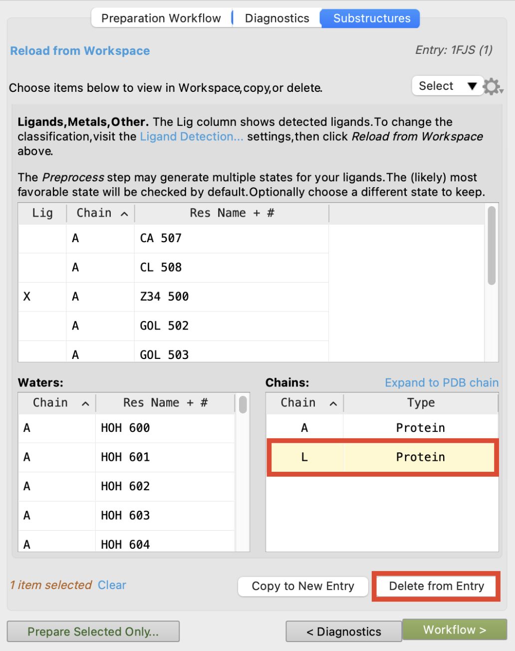
Figure 2-4. Review the structure for preparation in the Substructures tab.

Note

Unless specified, waters and glycerols (GOL) belonging to chain L will not be removed. Glycerols are a crystallographic artifact with no biological relevance. The Select dropdown provides shortcuts for selecting these species based on their proximity to specified chains. Removing waters and glycerols will be available again in the Minimize and Delete Waters step and in the Analysis step.

9. Select the Diagnostics tab and click Check Workspace Entry to see what kind of problems there are with our structure (The follwing figure indicates that One issue was found.)

• Valences: This tab lists atoms that have valence violations, such as missing hydrogens or the incorrect number of bonds.

• Missing: This tab lists residues for which atoms are missing.

• Overlapping: This tab lists pairs of atoms that are too close (bad contacts). When examining overlapping atoms, it is a good idea to ensure that all atoms are displayed. By default, only polar hydrogens are displayed, so you should select Show All Hydrogens from the hydrogens button menu in the Style toolbox, then open this dialog box. However, since structures downloaded from the PDB miss hydrogen atoms, one should first add hydrogens before addressing overlapping atoms.

• Alternates: This tab lists residues that have alternate positions in the input structure. Although these positions are legitimate, the protein preparation can only be done on a structure with a single set of coordinates, so you must choose one of the alternate positions for each residue. If you just intend to use this structure for docking, all we really need to care about are residues in the binding site, since Glide treats the receptor as rigid. To choose a position for a residue, go to Alternates tab and select the residue in the table. The view zooms in to the residue, the default position is marked, and the alternate position is drawn in with dotted lines. Click Switch to switch between positions (or use the check boxes in the Default and Alternate columns). When the position that you want to keep is displayed, click Commit. The atoms in this position are kept, and the alternate atoms are deleted.

Note

These issues can be usually addressed during subsequent protein preparation, but some default settings may not always be adequate, such as the position of residues in the binding site which should be carefully selected instead of keeping default.

10. Select Reports to view other issues with the protein that must resolved prior to modeling

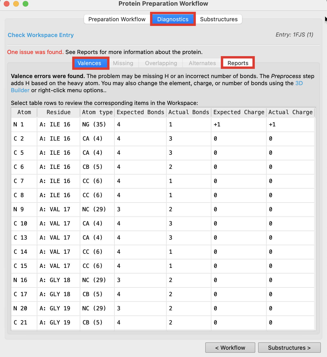
Figure 2-5. View protein issues in the Diagnostics tab

11. Return to the Preparation Workflow tab

12. Confirm Preprocess is toggled on

• Notice Fill in missing side chains is checked by default. If these were missing in our structure they would become populated during this step

13. Under Preprocess, select More Options

• Among the options provided, notice that missing loops may be filled in using Prime

14. Check the pH range for generating het states with Epik

• This should align with the physiological or assay pH.

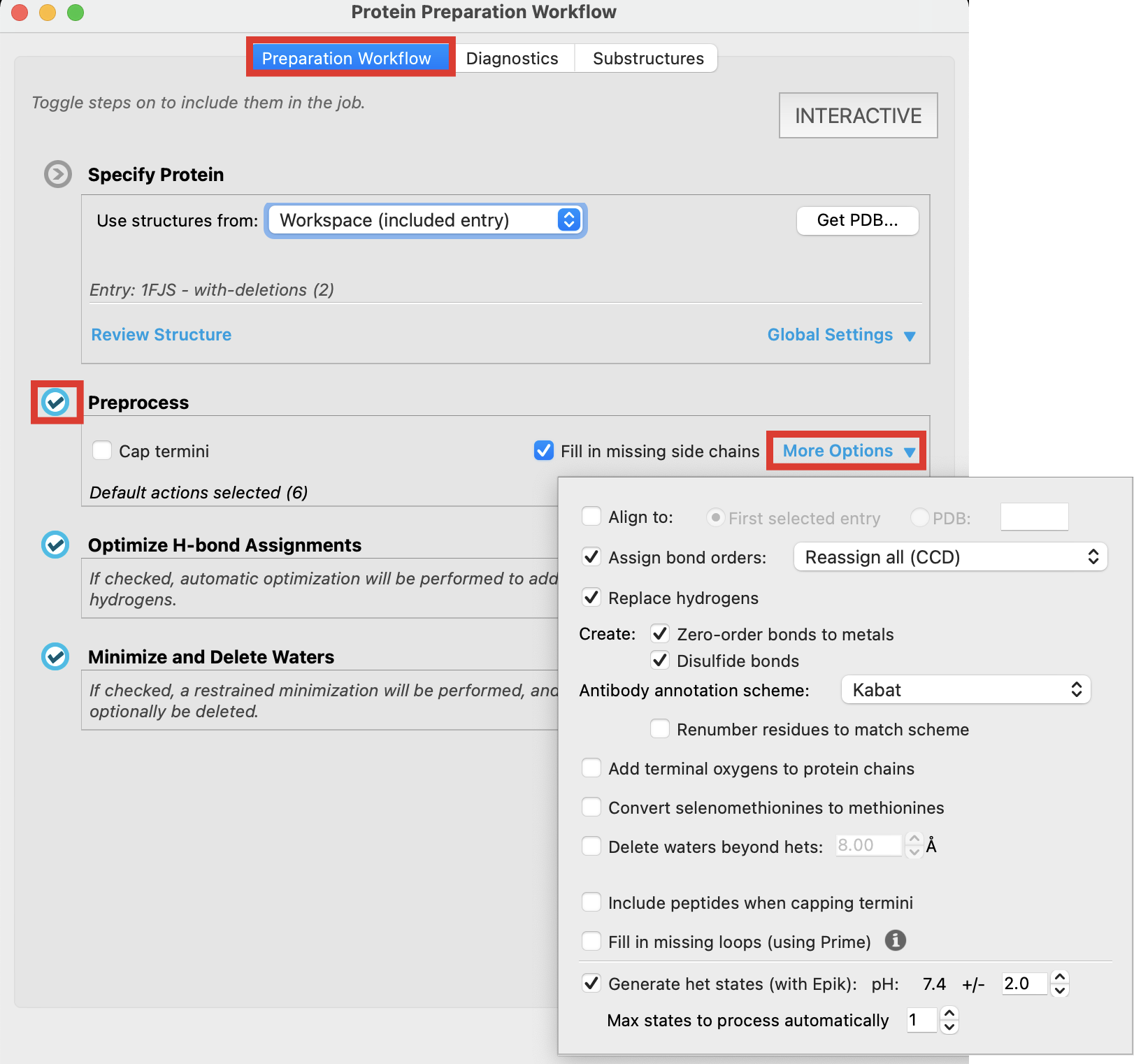
Figure 2-6. Preprocess default settings

Note

Preprocess Setting^{2, 3}

• Cap termini option

  • Add ACE (N-acetyl) and NMA (N-methyl amide) groups to uncapped N and C termini. These termini include any chain breaks where there are missing residues. If the chain breaks are far from the region of interest, it might be sufficient to cap them. If you want to fill in the chain breaks rather than cap them, select Fill in missing side chains.

• Fill in missing side chains option

  • Run a Prime refinement job to place and optimize the missing side chains.

• Align to options

  • Align the structure to another structure.

• Assign bond orders option

  • Assign bond orders to all bonds in the structure, including het groups. This option performs the same task as Edit → Assign → Bond Orders . It has some rules for assigning protonation states, but you should ensure that you have the correct states by selecting Generate het states (with Epik).

• Use CCD database option

  • Assign bond orders to het groups using the Chemical Components Dictionary (CCD). A SMARTS pattern is generated for the het group to look it up in the CCD. If the lookup fails, the bond order assignment is done with the default tools for assigning bond orders to structures. Note that this option does not assign ionization states, so if you use this option, be sure to also select

• Generate het states (with Epik)

  • The exception is ligands that are covalently bound to the protein, for which the default bond order assignment is used. In this case, the default assignment takes account of the covalent bonding and its consequences in the rest of the ligand, where use of the CCD would not.

• Replace hydrogens option

  • Remove the original hydrogens, then add hydrogens to the structure. This option allows any problems with hydrogen atoms in the original structure to be fixed. It includes fixing nonstandard PDB atom names, which prevent proper H-bond assignment, and is important for the H-bond optimization tool.

• Create options

  • Create bonds for specific structural features.

    • Zero-order bonds to metals—Break bonds to metals and correct the formal charge on the metal and the neighboring atoms to treat the bonds as ionic. This is required for use with force fields, which treat metal compounds as ionic rather than covalent. Then add zero-order bonds between the metal and its ligands, so that it is still considered part of the same molecule. Sulfurs that interact with metals have their hydrogens removed, if necessary, and are assigned a negative charge.

    • Disulfide bonds—Find sulfur atoms that are within 3.2 Å of each other, and add bonds between them. CYS residues are renamed to CYX when the bond is added.

• Antibody annotation scheme option menu

  • Select the annotation scheme to use for antibody structures, from the common schemes. The default scheme is Kabat. Information on the antibody structural regions is added to the structure as an atom property, antibody region id scheme. This information is used in the Structure Hierarchy to identify antibody regions for display and selection.

• Renumber residues to match scheme option

  • Renumber the residues to match the chosen antibody annotation scheme. By default the residue numbers are retained.

• Convert selenomethionines to methionines option

  • This option converts selenomethionines (MSE) to methionines (MET). A dialog box opens to inform you if any conversions are done. The conversion may be useful for structures in which MSE substitution was performed for X-ray structure determination.

• Delete waters beyond hets option and text box

  • Delete waters that are more than the specified distance (in angstroms) from any het group selected under Small molecules ("hets") to process. This is mainly useful for retaining waters that are important for ligand binding, while deleting all other waters.

  • For docking, and any other applications that critically depend on binding site volume, it is recommended to keep waters until the Minimize and Delete waters step, to ensure that the binding site retains its volume.

  • You can delete waters individually in the Substructures tab, and you can delete waters that do not form H-bonds with non-waters or are distant from het groups (same as this option) in the Minimize and Delete waters step.

• Fill in missing loops (using Prime) option

  • This option will build and add loops of up to 20 residues, but not tails or terminal regions. After the structure is prepared, newly created loops should be refined to improve their quality. The first attempt at loop building is made using a knowledge-based approach. If this approach fails, a subsequent attempt will use an energy-based approach. Built-in loops can be identified by selecting atoms based on the atom property b_psp_added_missing_loops. (Release 2023-4)

  • Fill in missing loops from the SEQRES records in the PDB file, using the Prime refinement program. Only short loops are filled in. For longer loops, you can use protein crosslinking (see Crosslink Proteins Panel) or homology modeling (see Build Homology Model Panel) to fill in a loop. The resulting loop may not be of high quality, and a full Prime loop refinement can be performed to obtain higher quality. See the Refine Loops Panel topic for details. If the missing residues are far from the site of interest, it might be sufficient to cap them by selecting Cap termini. (Not available from Maestro Elements.) (Release 2022-4)

• Generate het states (with Epik) option

  • Run Epik to generate probable ionization and tautomeric states in the pH range specified for all selected het groups, as well as states prepared for binding to metals if the het group is coordinated to a metal. This ensures that the ligands have the proper ionization and tautomeric state, which might not be assigned when using the CCD database for bond orders.

    • pH value and range text box

      • For the target pH specified under Global Settings (and reported here), set the pH range for the generation of probable ionization and tautomeric states in the text box.

    • Max states to process automatically text box

      • When running the protein preparation automatically as a job, specify the number of het states to return for each protein processed. The states are selected in order of increasing state penalty. If you are running the preparation interactively, you can view and select the het states in the Substructures Tab.

Note

Het groups are everything that is not a water or a protein residue, and include ligands, metal ions, and cofactors. Chains are defined by the chain label, and can include waters and het groups.⁴

15. Confirm Optimize H-bond Assignment is toggled on

16. Click Settings

• Overlapping atoms caused by the addition of hydrogens during the Preprocess step will be corrected, and side chains may be flipped when this job is run

Note

If you have a lot of water molecules in the structure, sampling can take a long time. You should ensure that you have deleted unwanted waters before you start this process (e.g. Check the Delete waters beyond hets option in Preprocess).

17. Check the pH for Optimization

• This value should be captured in the pH range chosen during the Preprocess step

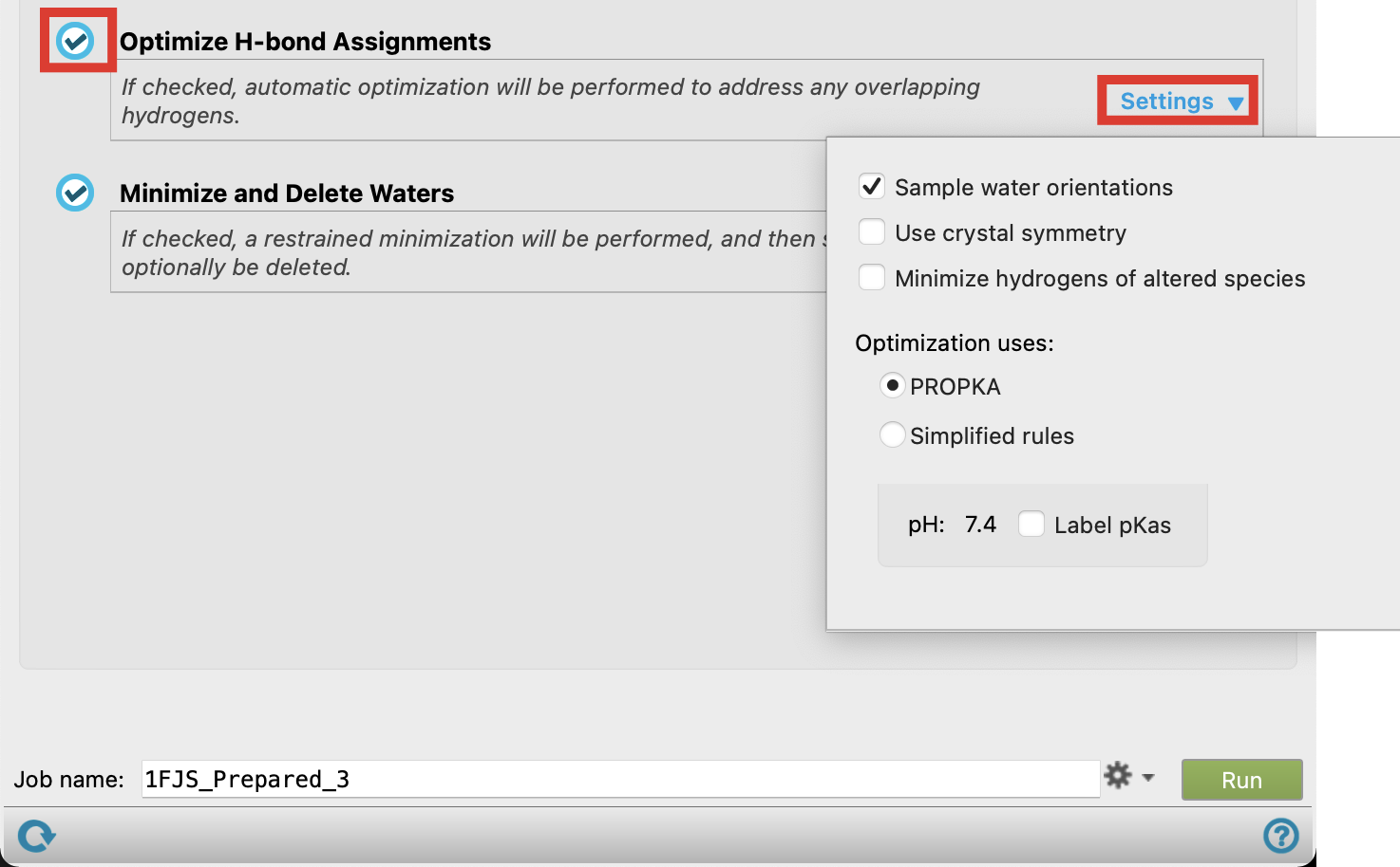
Figure 2-7. Optimize H-Bond Assignment default settings

Note

For more information on Optimize H-bond Assignments, please refer to here.

18. Confirm Minimize and Delete Waters is toggled on

19. Click Settings

• Notice that by default distant waters will not be removed. The specified distance to ligands can be modified

20. Change the job name to 1FJS_Prepared

21. Click Run

• This job will take a few minutes as all toggled jobs are running consecutively

• A new group will be added to the Entry List

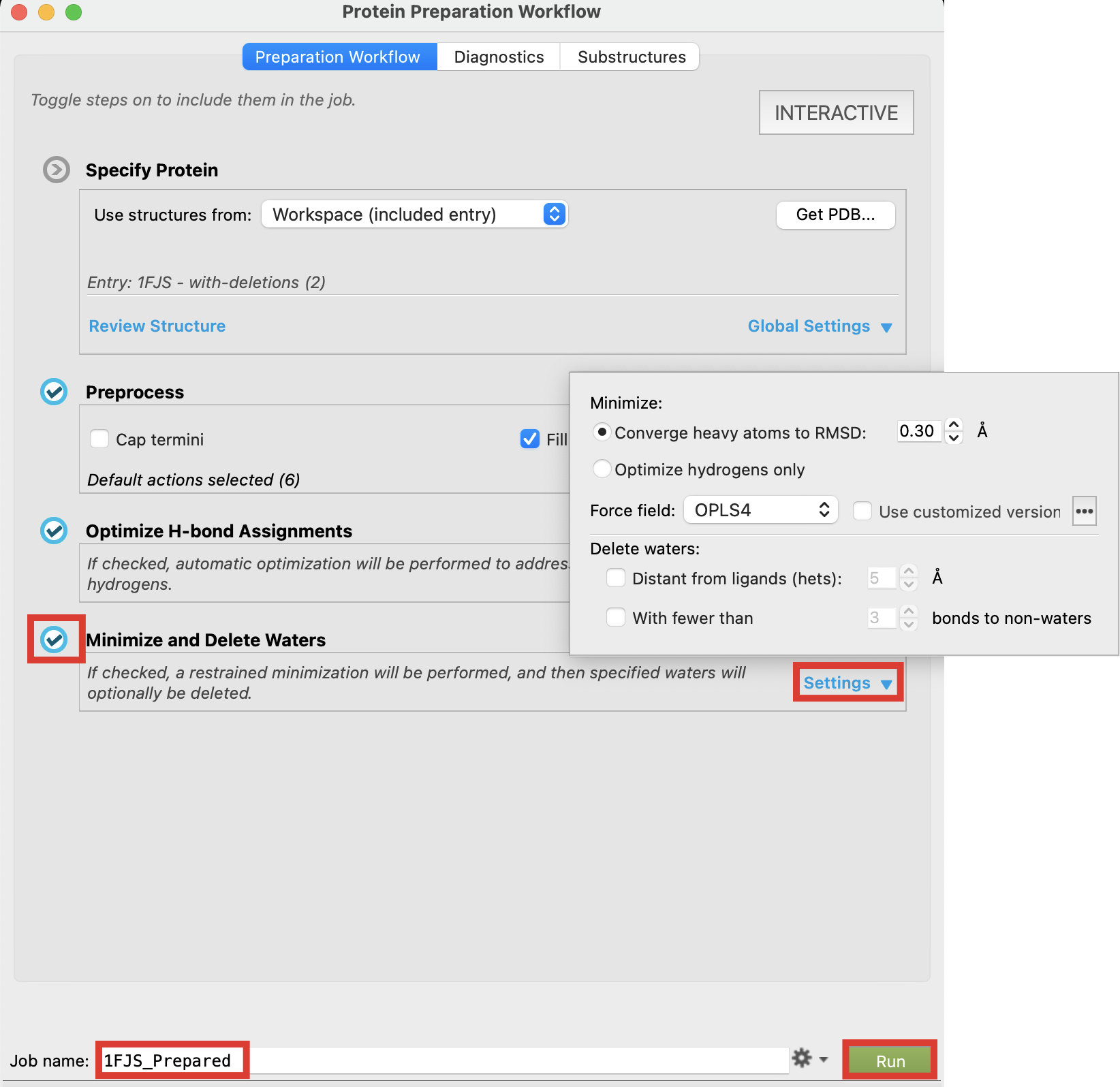
Figure 2-8. Minimize and Delete Waters default Settings

22. In the Entry List, Include and Select 1FJS – prepared

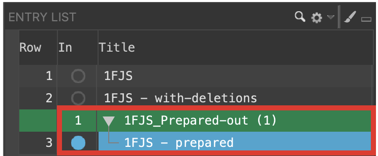
Figure 2-9. Select the protein preparation output

Note

In Interactive mode, multiple entries will be added to the Entry List as each individual preparation task will be run as an independent job.

23. Return to the Protein Preparation tool

24. Click the Substructures tab and click Reload from Workspace

25. In the Hets table, shift-click to select all GOL rows and click Delete from Entry to delete glycerol molecules from the structure

26. In the Waters table, shift-click to select all waters and click Delete from Entry to deldte water molecules form the structure

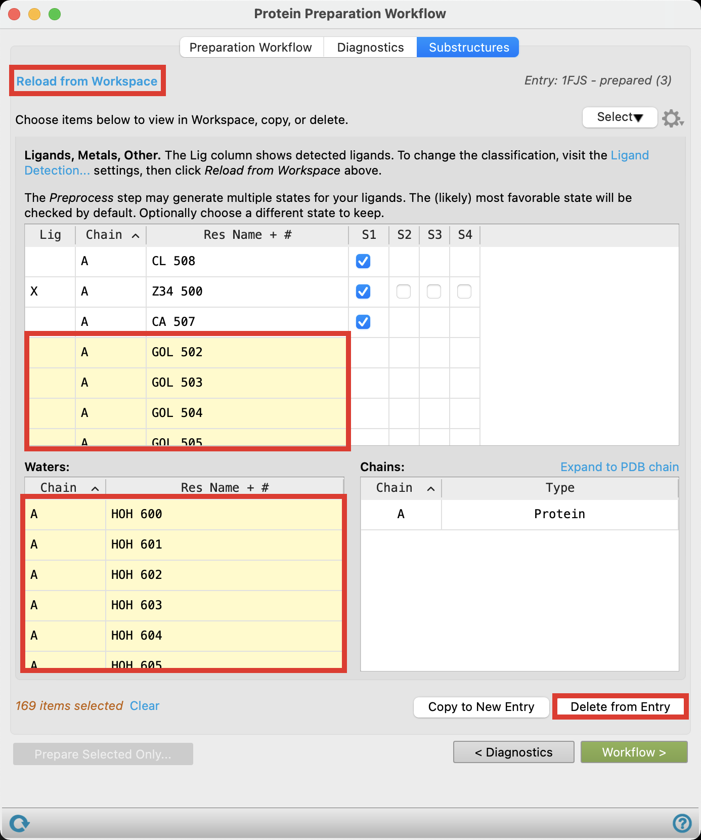
Figure 2-10. Perform Substructure Review

Note

These waters could have been removed during the Minimize and Delete Waters processing step. Again, depending on your system and research question, you may want to keep certain waters. See the Protein Preparation Workflow Panel Documentation as well as this Knowledge Base Article for more details.

27. Notice that in the 1FJS_Prepared-out1 group, you now have 1FJS – with-deletions included

28. Return to the Protein Preparation Workflow and click the Diagnostics tab to make sure there are no issues missed during the preparation. You may need to click Check Workspace Entry

29. Exit the Protein Preparation Workflow

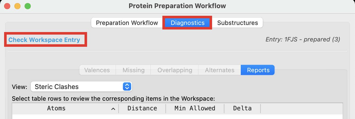
Figure 2-11. Confirm issues have been resolved during preparation

If issues persist after preparation, perform specific interactive protein preparations on the modified protein with adjusted settings. The job type will depend on which problems were found.

Generating a Receptor Grid using the Receptor Grid Generation

This section is based on the article, “Structure-Based Virtual Screening Using Glide”4, and created with the Schrödinger Software Release 2023-4.

Grid generation must be performed prior to running a virtual screen with Glide. The shape and properties of the receptor are represented in a grid by fields that become progressively more discriminating during the docking process. To add more information to a receptor grid, different kinds of constraints can be applied during the grid generation stage. For a comprehensive overview of constraint options, see the Glide User Manual. In this section, setting a hydrogen bond constraint in the receptor grid is shown. In Section 5, additional types of constraints (i.e. core constraint) are discussed.

1. Import 1fjs_prep_complex and include

• The "1fjs_prep_complex" is a renamed version of the "1FJS – with-deletions" entry that was generated in the "Prepare the Protein using the Protein Preparation Workflow" section ( Step 27), you can also directly download it on here.

2. Double-click Presets

• 1fjs_prep_complex is rendered using the Custom Preset

3. Go to Tasks > Browse >  Receptor-Based Virtual Screening > Receptor Grid Generation

• The Receptor Grid Generation panel opens

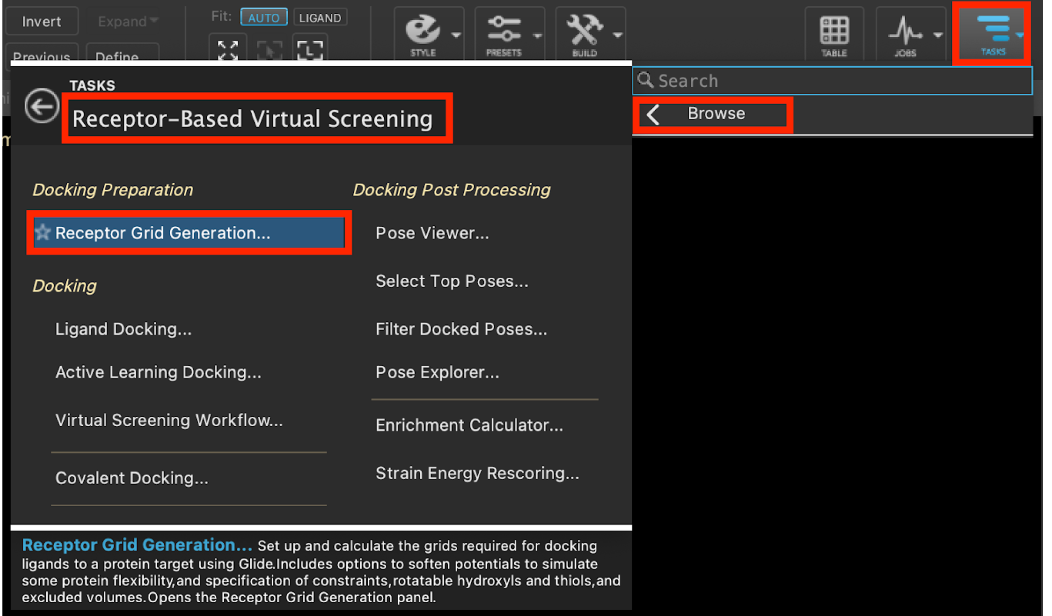
Figure 3-1. Receptor Grid Generation option in Receptor-Based Virtual Screening.

4. Under Define Receptor, check the boxes for Pick to Identify the ligand (Molecule) and Show Markers

• A banner in the Workspace will prompt you to click on an atom in the ligand

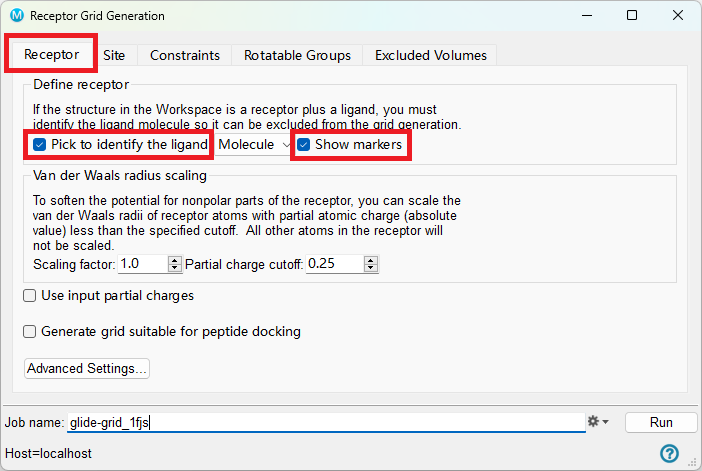
Figure 3-2. The Receptor tab of Receptor Grid Generation.

5. Click on the ligand

• The ligand is now highlighted with a purple box around it

• The ligand will be excluded from the grid generation

Note

The purple bounding box defines the region that the docked molecule(s) can occupy to satisfy the initial stages of docking.

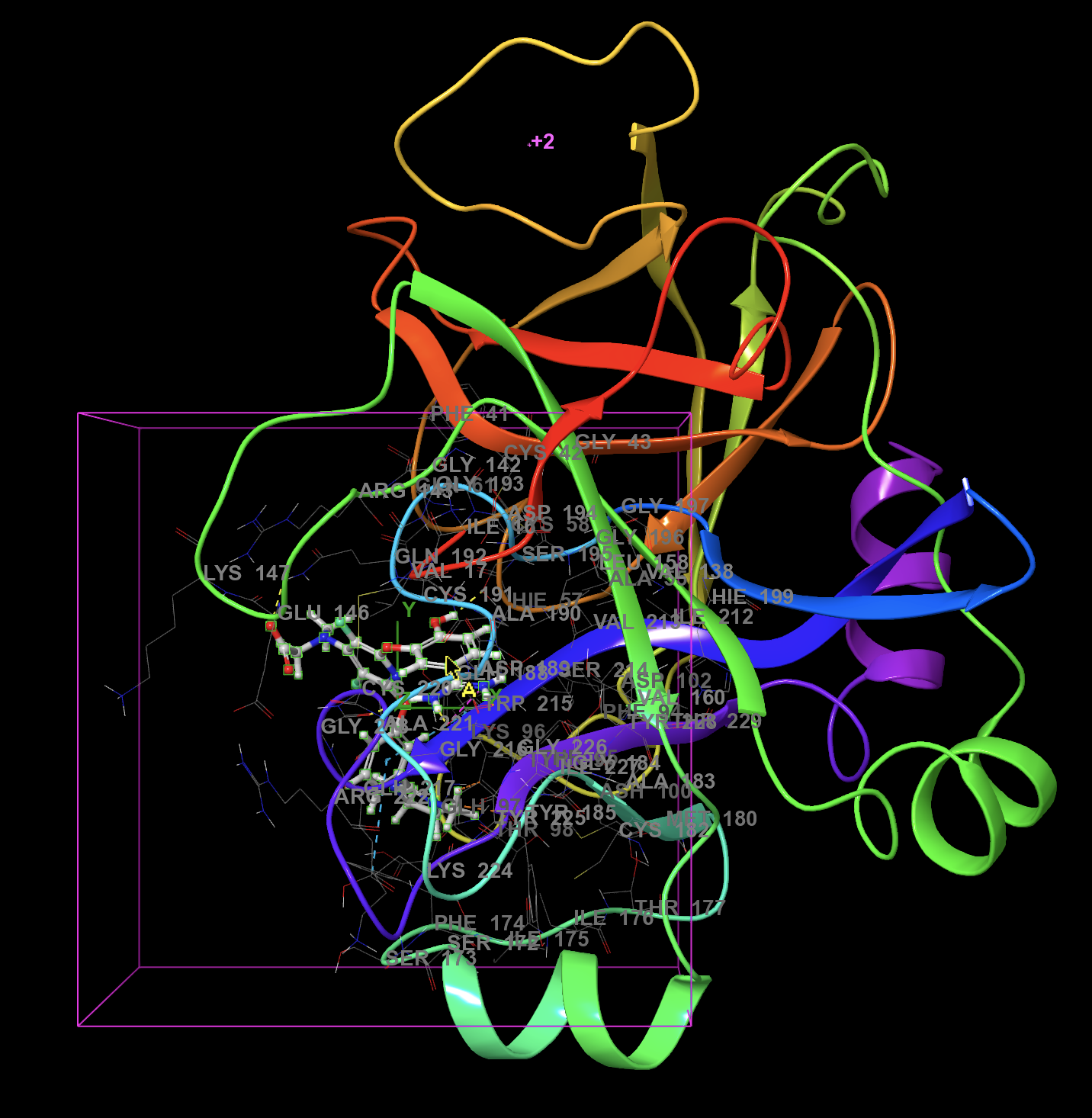
Figure 3-3. The ligand is defined to be excluded from grid generation.

Note

Van der Waals radius scaling section⁵

• Glide does not allow for flexible receptor docking (apart from hydroxyl rotations). However, scaling of van der Waals radii of nonpolar atoms, which decreases penalties for close contacts, can be used to model a slight "give" in the receptor and the ligand. (Receptor flexibility can be modeled with Glide/Prime Induced Fit docking—see Induced Fit Docking). You can use the features under Van der Waals radii scaling to scale the van der Waals radii of those receptor atoms defined as nonpolar by a partial charge threshold you can set. For ordinary Glide docking, it is recommended that receptor radii be left unchanged, and any scaling be carried out on ligand atoms. Receptor scaling is probably most useful when the active site is tight and encapsulated. information on scaling of vdW radii of nonpolar ligand atoms, see the Ligand Docking Panel topic.

• Scaling factor text box

  • This text box specifies the scaling factor: van der Waals radii of nonpolar receptor atoms are multiplied by this value. The default value is 1.00, which means that the receptor atom radii are not scaled.

• Partial charge cutoff text box

  • Scaling of vdW radii is performed only on nonpolar atoms, defined as those for which the absolute value of the partial atomic charge is less than or equal to the number in the text box. Since this is an absolute value, the number entered must be positive. The default for receptor atoms is 0.25.

6. Click the Site tab

7. Select Centroid of Workspace ligand (selected in the Receptor tab)

• Centroid of Workspace ligand (selected in the Receptor tab): Center grids at the centroid of the ligand molecule that was selected in the Receptor tab. This ligand should be in the Workspace. If such a ligand has been selected, this option is the default. The Advanced Settings button is available with this option.

• Centroid of selected residues: Center grids at the centroid of a set of residues that you select. With this option you can define the active site (where grids should be centered) with only the receptor in the Workspace. The Specify Residues button is only available when you choose this option; the Advanced Settings button is not available with this option. The Specify Residues button opens the Active Site Residues Dialog Box, in which you can pick the residues that best define the active site.

• Supplied X, Y, Z coordinates: Center grids at the specified coordinates. Center the grid at the Cartesian coordinates that you specify in the X, Y, and Z text boxes. The coordinates of the grid center chosen by any of the other two methods are displayed in these text boxes. These text boxes are only available when you choose this option. The Advanced Settings button is available with this option.

8. Click Advanced Settings

• A green inner bounding box appears

Note

The green bounding box defines the region in which the centroid of the docked molecule(s) must occupy to pass the initial stages docking

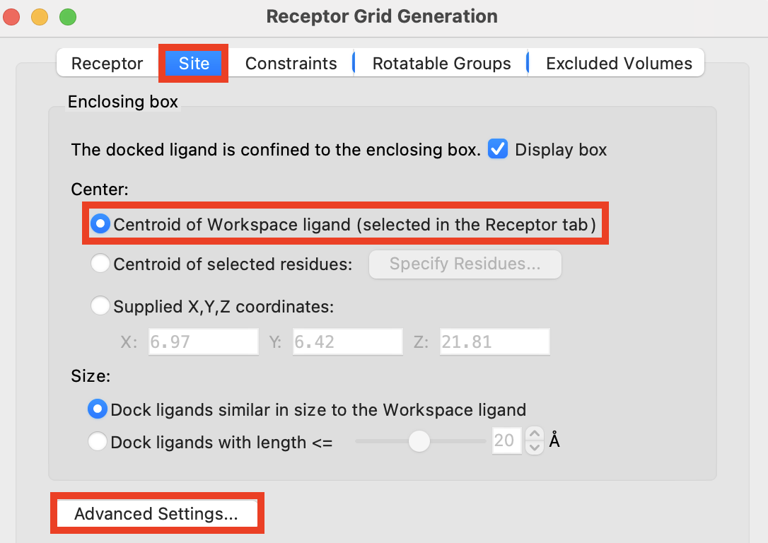
Figure 3-4. The Site tab of Receptor Grid Generation.

Note

The diameter midpoint of each docked ligand is required to remain within smaller, nested box depicted in green.

9. Keep the default settings for X, Y, and Z sizes the same at 10 Å, 10 Å, and 10 Å, respectively.

10. Click OK

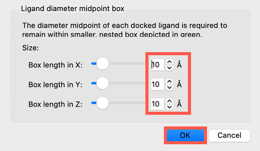
Figure 3-5. Ligand diameter midpoint box panel.

11. Click Fit to ligand view to zoom to the ligand

12. In the Structure Hierarchy, click the magnifying glass

13. In the search field, type ASP 189

14. Select ASP 189

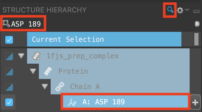
Figure 3-6. Search in the Structure Hierarchy.

Note

According to Adleret al., the salt bridge formed between the inhibitor and Asp189 observed in the crystal structure of the complex contributes to the potency of the ligand. For this tutorial, you will set the constraint for this specific hydrogen bond in the receptor grid. Please see the Introduction to Structure Preparation and Visualization tutorial for instructions on how to add residue labels and show H-bonds.

15. Under Fit, click Fit view to selected atoms

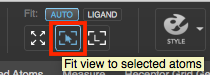
Figure 3-7. Zoom to selected atoms.

16. In the Receptor Grid Generation panel, click the Constraints tab

17. Click the H-bond/Metal (0) tab

• A banner appears prompting selection of the receptor atom to be the constraint

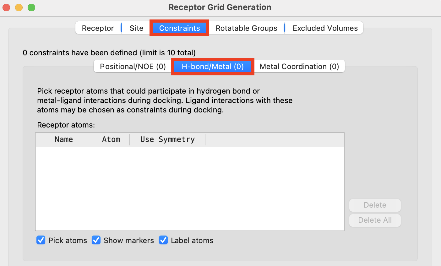
Figure 3-8. The Constraints tab of Receptor Grid Generation.

18. Click an oxygen atom of the ASP 189 sidechain

• Both oxygens are highlighted

• An H-bond constraint is defined in the Receptor atoms table

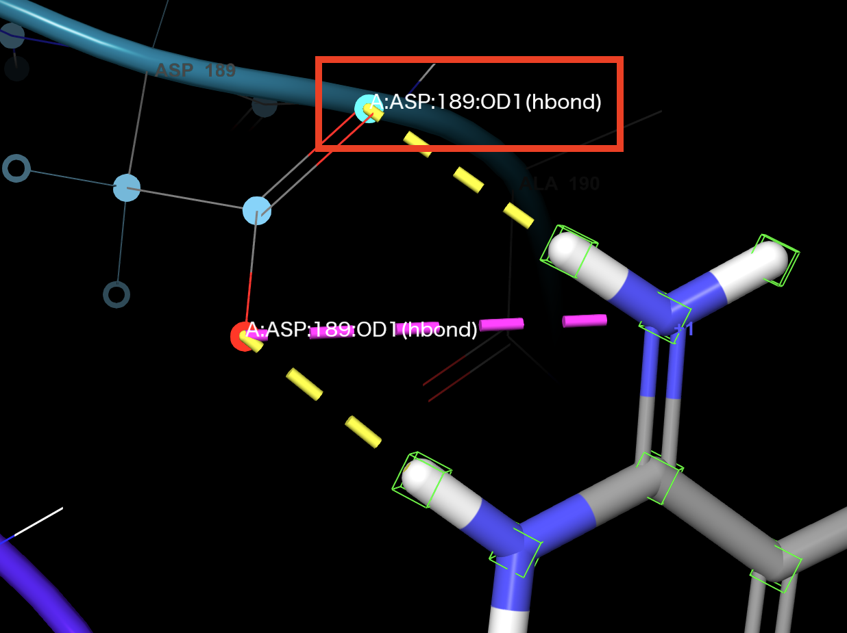
Figure 3-9. Constraint defined on ASP 189.

19. Change Job name to glide-grid_1fjs

20. Click Run

• This job will take about a minute

• A folder named glide-grid_1fjs is written to your Working Directory

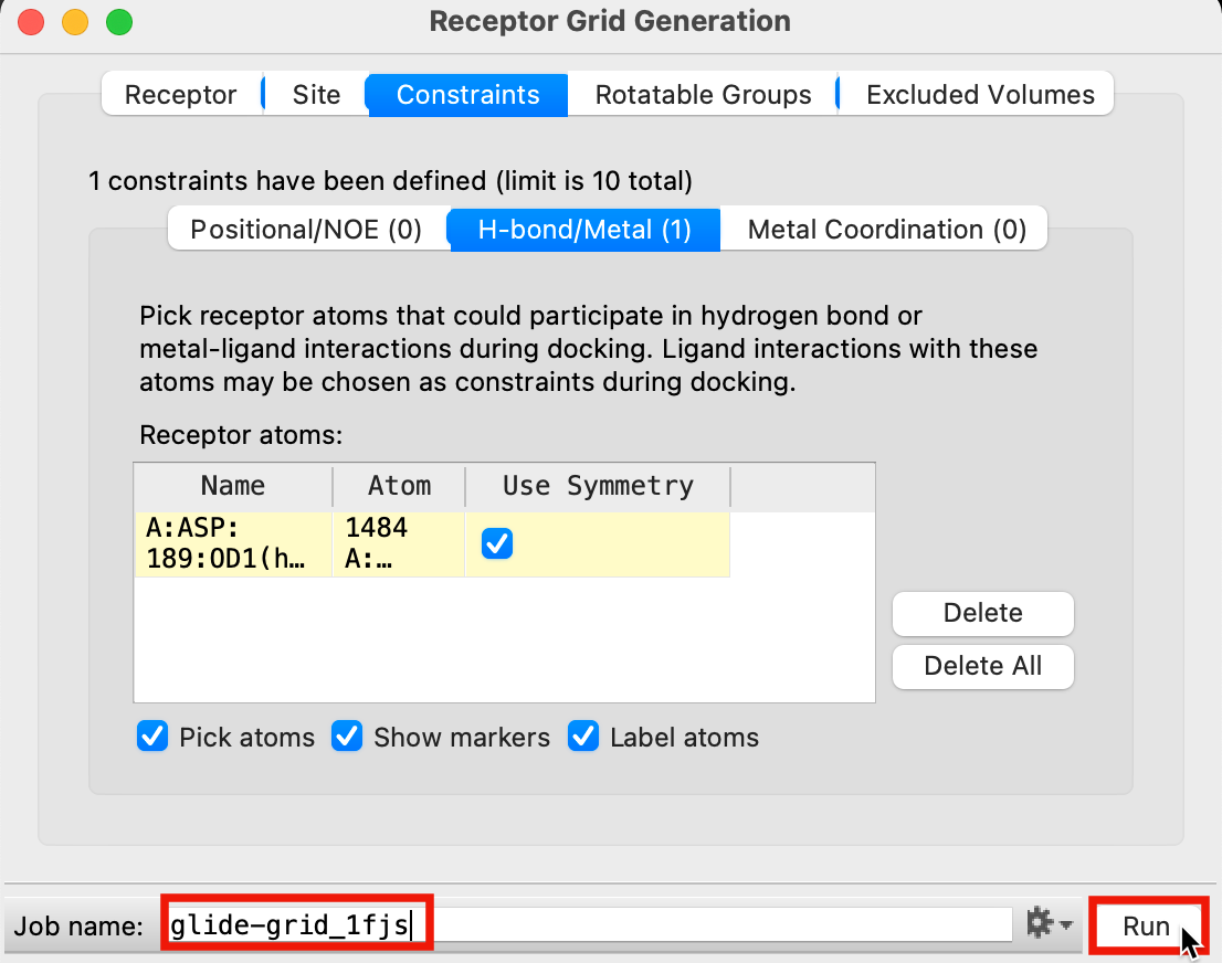
Figure 3-10. Run receptor grid generation job.

Preparing a Ligand Structure Using the LigPrep

This section is based on the article, “Introduction to Structure Preparation and Visualization”1, and created with the Schrödinger Software Release 2023-4.

1. Import 1FJS_prepared_dry_ligand and include

• 1FJS_prepared_dry_ligand is the ligand was extracted from 1fjs_prep_complex, you can directly download it on here.

2. Go to Tasks > Browse > LigPrep

• The LigPrep panel opens

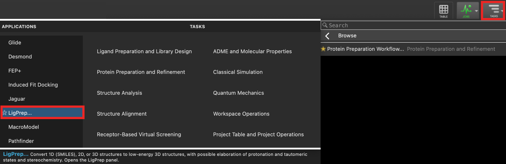
Figure 4-1. LigPrep application in the Task toolbar.

3. For Use structures from, choose Workspace (1 included entry)

4. Under Stereoisomers, choose Determine chiralities from 3D structure

5. Change Job name to ligprep_1fjs

6. Click Run

• A banner appears when the job has been incorporated

• A new group is added to the Entry List

• The number of ligands in this group is shown in parentheses

Figure 4-2. The LigPrep panel.

Note

The number of structures produced can vary a great deal, depending on the ligands being processed. The factors affecting the number of structures produced are described below:

• In the Ionization section, only Generate possible states at target pH should increase the number of structures. The increase is typically a factor of approximately 1.4 for a pH range of 2.0. Reducing the pH range significantly reduces this factor.

• The Generate tautomers option typically increases the number of structures by less than 20%.

• In the Stereoisomers section, only Generate all combinations should result in many more structures. For individual ligands the increase can be as large as 2n, where n is the number of chiral centers. For large data sets the increase is typically around 1.5, but is very dependent on the classes of molecules being processed. You can reduce the number of structures produced by entering a smaller value in Generate stereoisomers (maximum), however this does increase the risk of missing important stereoisomers.

7. Type Ctrl+T (Cmd+T) to open the Project Table, or select Table in the upper right hand of Maestro
8. Click Tree to open the Property Tree

• Different calculated properties can be toggled on and off

• Click the arrow next to each application to view more properties

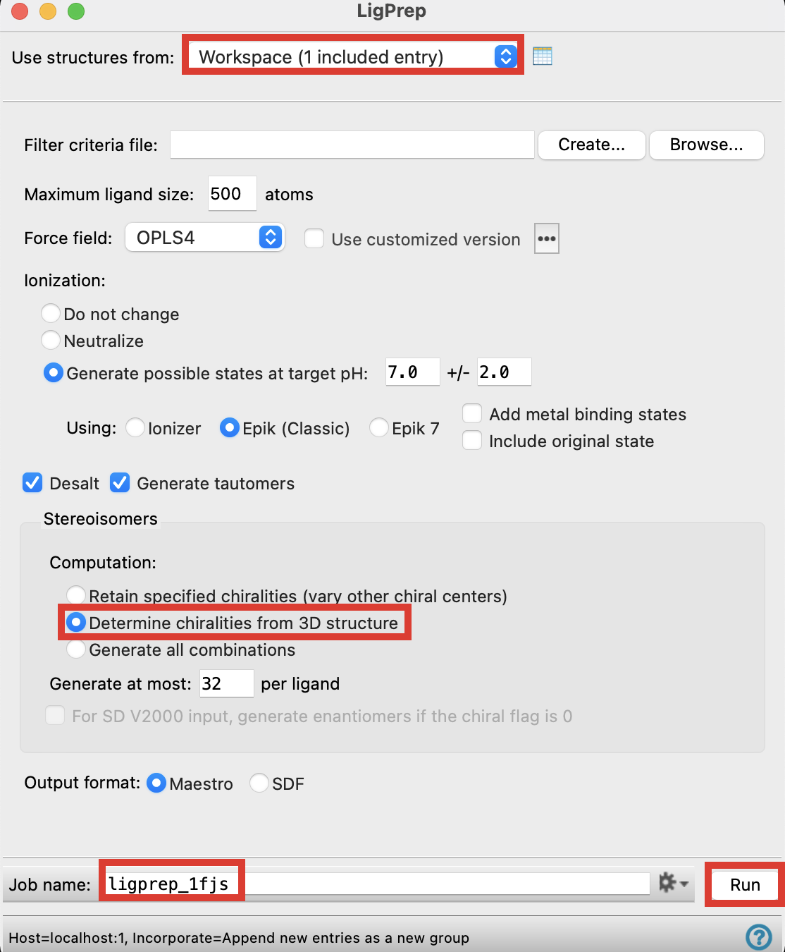
Figure 4-3. The Project Table with the Property Tree open.

Note

For more information about LigPrep, please refer to LigPrep Panel (schrodinger.com).

Dock the Ligand

This section is based on the article, “Structure-Based Virtual Screening Using Glide”4, and created with the Schrödinger Software Release 2023-4 on Windows 11.

In this tutorial, we will dock the ligand extracted from the protein complex, which is usually assumed to be the cognate ligand, means the ligand bound in a crystal structure or some other structure that is used in a positive control docking experiment.

1. Go to Tasks > Browse > Receptor-Based Virtual Screening > Ligand Docking

• The Ligand Docking panel opens

2. Next to Receptor grid, click Browse and choose glide-grid_1fjs.zip generated by previous steps

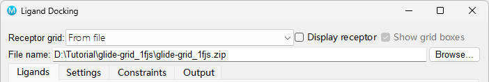
Figure 5-1. Importing the receptor grid files for docking.

3. A new window will appear verifying that receptor constraints were found in the receptor grid. Click OK.

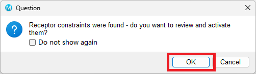
Figure 5-2. A window that verifies receptor constraints.

4. This takes you to the Constraints tab. Click on the Receptor tab.

5. Under Use, check the H-bond constraint for ASP 189

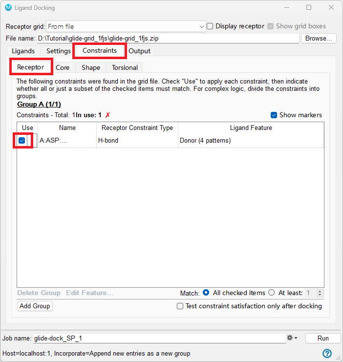
Figure 5-3. The Constraints tab of the Ligand Docking panel.

6. In the Ligands tab, for Use ligands from, choose Files

7. Next to File name, click Browse and choose ligprep_1FJS-out.maegz

8. Keep the other options default unless otherwise requested in the Ligands tab

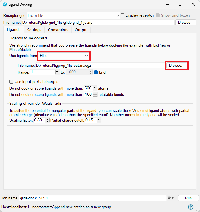
Figure 5-4. The Ligands tab of the Ligand Docking panel.

Note

Use input parital charges sections: Select this option to use partial charges from the input structures instead of those automatically assigned by the OPLS force field at run time. It is recommended using the default charges assigned by the force field, unless you find they are inadequate in some way, or you have alternative high-quality charges (e.g., from QM) that you wish to use instead.

Scaling of van der Waals radii section: To soften the potential for nonpolar parts of the ligand, you can scale the vdW radii of ligand atoms with partial atomic charge (absolute value) less than the specified cutoff (the default for ligand atoms is 0.15). The Scaling factor text box specifies the scaling factor,and the default is 0.80. To turn van der Waals radii scaling off, set the scaling factor to 1.0.

9. Go to the Settings tab and keep all options default unless otherwise requested

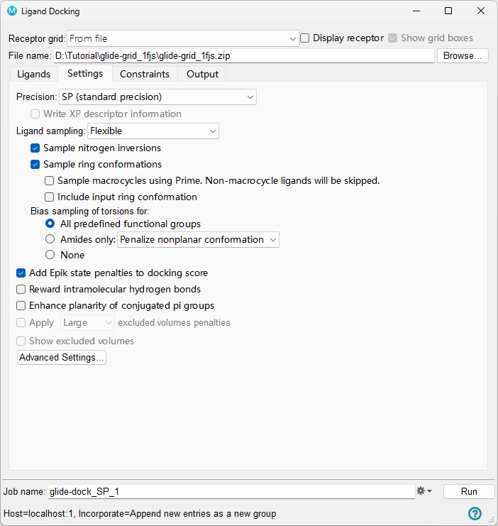
Figure 5-5. The Settings tab of the Ligand Docking panel.

Note

Settings tab

• Precision option menu—Choose a docking precision:

  • HTVS (high throughput virtual screening): HTVS docking is intended for the rapid screening of very large numbers of ligands.

  • SP (standard precision): SP docking is appropriate for screening ligands of unknown quality in large numbers.

  • XP (extra precision): XP docking and scoring is a more powerful and discriminating procedure, which takes longer to run than SP. XP is designed to be used on ligand poses that have been determined to be high-scoring using SP docking. It is recommended that you run your database through SP docking first, then take the top 10% to 30% of your final poses and dock them using XP, so that you perform the more expensive docking simulation on worthwhile poses.

  • SP-Peptide: Standard-precision docking for peptide ligands uses the same general settings as for regular standard precision but changes some of the settings to enhance the retention of poses. If you select this option, the grid must be one that was generated for this mode, i.e. with Generate grid suitable for peptide docking selected in the Receptor tab of the Receptor Grid Generation panel.

• Ligand sampling option menu and options—The Ligand sampling option menu allows you to choose whether ligands are docked flexibly, rigidly, or not at all (score in place).

  • Flexible: This is the default choice and directs Glide to generate conformations internally during the docking process; this procedure is known as "flexible docking". Conformation generation is limited to variation around acyclic torsion bonds, sampling of low-energy ring conformations, and generation of pyramidalizations at certain trigonal nitrogen centers, e.g. in sulfonamides. For a set of predefined functional groups, such as amides and esters, you can bias sampling of the torsion around the bond that normally adopts a particular conformation so that it adopts the desired conformation. There are several options for conformation generation with this choice:

    • Sample nitrogen inversions option: Sample inversions at pyramidal nitrogen atoms (not amides). This option is selected by default.

    • Sample ring conformations option: Sample the conformations of rings, using the same technology as in LigPrep—see Ring Conformations: ring_conf for details. These conformations are not sampled in the main conformation generation, which focuses on sampling of rotatable bonds, leaving the core fixed. Deselect this option if you want rings to remain in their input conformations throughout docking.This option is selected by default. The two following options are made available if this option is selected.

      • Sample macrocycles using Prime option: Sample the conformations of macrocycles using the Prime macrocycle sampling code (see Prime Macrocycle Sampling Panel), with special options for Glide docking.

      • Include input ring conformation option: Select this option if you want to include the input conformations of rings in addition to other conformations. The conformational sampling uses the input conformation as a seed, and does not necessarily include it in the set of conformations returned.

    • Bias sampling of torsions for options: Choose an option for sampling of torsions that should normally be restricted to a particular conformation. The biasing can include retention of the input conformation, setting the torsion to a particular value, applying a penalty for deviating from the desired conformations, or allowing only a particular conformation to within a small angle range. The options cover different selections of functional groups:

      • Predefined functional groups: Bias the sampling of torsions for a set of functional groups that is defined in a resource file (default). The choice of biasing method, as outlined above, is set in the resource file. The resource file can be customized—see Customizing Torsional Controls for Docking Planar and Other Groups.

      • Amides bonds only: This option applies constraints or penalties to rotation around amide C–N bonds. The option menu provides a choice of the constraint type:

        • Penalize non-planar conformation—penalize amide bonds that are not cis or trans (default)

        • Retain original conformation— freeze amide bonds in their input conformation throughout docking

        • Allow trans conformation only—enforce trans conformation within a small angle range (20°). Ligands that do not dock in this range are rejected.

      • None: Do not penalize or constrain rotations about certain bond types, but allow them to adopt a conformation according to the force field.

    • Rigid: Rigid docking allows the existing ligand structure to be translated and rigidly rotated relative to the receptor, but skips the conformation generation step.

    • None (refine only): With this option, the input ligand structure does not pass through the Glide docking procedure, but the input coordinates are used to perform an optimization of the ligand structure in the field of the receptor, and then the ligand is scored. The goal of this docking method is to find the best-scoring pose that is geometrically similar to the input pose. For HTVS and SP, a minimization is performed; for XP, the ligand is regrown in place. With XP mode, this option is not a substitute for a full XP docking calculation: XP mode requires accurate initial poses.

    • None (score in place only): When this option is selected, Glide does no docking, but rather uses the input ligand coordinates to position the ligands for scoring. It therefore requires accurate initial placement of the ligand with respect to the receptor. This option is useful to score the reference ligand in its cocrystallized or modeled position, or as a post-processing step on Glide-generated poses to obtain individual components of the GlideScore prediction of the binding affinity. It can also be used to check whether the scores of the known binders in their native proteins are similar enough to their scores when cross-docked to the chosen receptor protein. If this is the case, it is reasonable to expect that similar structures would also score well. This option should not be used with Glide XP, as full XP sampling is normally needed to avoid strong XP penalties for ligands that should be able to dock correctly.

• Add Epik state penalties to docking score option: If the ligands have been prepared using Epik for ionization and tautomerization, the Epik penalties for adopting higher-energy states (including those where metals are present) are added to the docking score when this option is selected. Ligands that do not have this information are not penalized and will therefore have better scores, so you should ensure that the ligand set is consistent. If the ligand interacts with a metal (distance less than 3.0 Å), the metal penalties that are computed when Epik is run with the metal binding option are used. If multiple ligand atom-metal interactions are found, the smallest value of the metal-specific penalty is used.

• Reward intramolecular hydrogen bonds option: Add a reward for each intramolecular hydrogen bond to the GlideScore. A contribution is also added to Emodel for each intramolecular H-bond, to favor selection of poses with intramolecular H-bonds. Ligands with intramolecular hydrogen bonds pay a smaller entropic penalty upon binding, so forming intramolecular H-bonds can be important for binding.

• Enhance planarity of conjugated pi groups option: Increase the torsional potential around bonds between atoms whose geometry should be planar (i.e. sp2 atoms). This option should make aromatic rings, amides, esters, and so on, less likely to adopt a nonplanar geometry. Nonplanarity of these groups is a physically reasonable effect, because the torsional potential has a finite barrier which can be overcome+ to some extent by other interactions. However, in Glide docking, nonplanarity can also be a result of the approximations made to reduce clashes with the receptor. To some extent, planarity can be enforced in flexible docking by choosing one of the biasing options for sampling torsions. However, if you want to improve planarity in post-docking minimization or for non-flexible docking, you should select this option.

• Apply excluded volumes penalties option and menu: If the grid has excluded volumes associated with it, select this option to apply all the excluded volumes, and choose the penalty level from the option menu. The penalty is applied if any ligand has atoms within the excluded volume. The value of the penalty ramps up from zero at the boundary of the volume to the maximum penalty at 90% of the sphere radius . The penalty is applied in both the rough scoring stage and the final docking

• Show excluded volumes option: Display in the Workspace the excluded volume spheres that are associated with the grid. Only available if the grid has excluded volumes and Apply excluded volumes penalties is selected.

• Advanced Settings button: Click this button to open the Settings- Advanced Settings Dialog Box. This dialog box provides options for ligand conformer generation, selection of initial poses, energy minimization, and inclusion of aromatic H-bonds and halogen bonds.

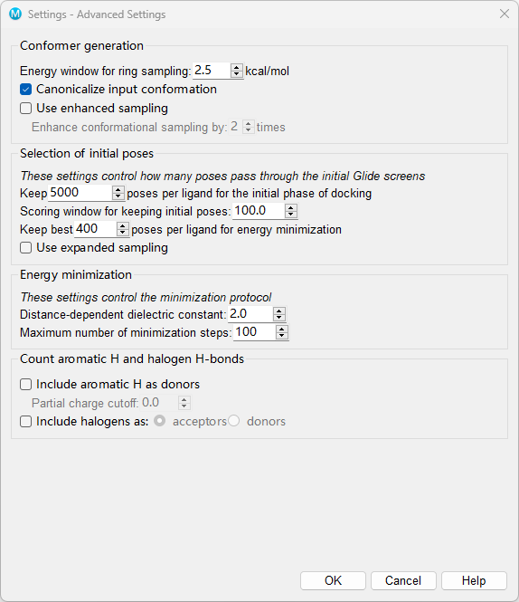
Figure 5-6. A window of Settings - Advanced Settings Dialog Box.

Settings - Advanced Settings Dialog Box

• Conformer generation section: This section contains settings related to the generation of conformers of each ligand.

  • Energy window for ring sampling text box The threshold for keeping or discarding ring conformations can be set in this text box. Ring conformations are discarded if their energies are higher than that of the lowest conformation by more than the amount specified.

  • Canonicalize input conformation option Ensure that the same starting conformation is always used for a given ligand, regardless of the input conformation or orientation, so that the output poses do not depend on details of the input structure. This is done by generating a new set of coordinates for the ligand based only on the connectivity and stereochemistry. The poses obtained in docking can depend on details of the input structure. Sometimes this is useful, to obtain a wider range of poses, but it can also prevent comparisons between docking runs that should not depend on the detailed structure of the input ligands.

    • Use enhanced sampling option Enhance the sampling of conformational space by adding variations on the input structure to the conformational search.

      • Enhance conformational sampling by N times text box Enhance the conformational sampling by the factor specified in the text box. This is done by generating variations on the input structure, and using these as seed structures along with the input structure for conformational sampling.

• Selection of initial poses section: The options in this section control the way poses pass through the filters for the initial geometric and complementarity fit between the ligand and receptor molecules. The grids for this stage contain values of a scoring function representing how favorable or unfavorable it would be to place ligand atoms of given general types in given elementary cubes of the grid. These grids have a constant spacing of 1 Å. The rough score for a given pose (position and orientation) of the ligand relative to the receptor is simply the sum of the appropriate grid scores for each of its atoms. By analogy with energy, favorable scores are negative, and the lower (more negative) the better. The initial rough scoring is done on a coarse grid, on which the possible positions for placing the ligand center are separated by 2 Å, twice the elementary cube spacing, in X, Y, and Z. The refinement step rescores the successful rough-score poses after the particular rigid translational repositioning of -1, 0, or +1 Å in X, Y, and Z, which gives the best possible score. This procedure effectively doubles the resolution of the scoring screen.

  • Keep n initial poses per ligand for the initial phase of docking: This text box sets the maximum number of poses per ligand to pass to the grid refinement calculation. The default setting depends on the type of docking specified and whether Glide constraints have been applied:

    • 5000 poses for flexible docking jobs in general.

    • 500 poses for flexible docking jobs to which Glide constraints are applied.

    • 1000 poses for rigid docking jobs (Glide constraints do not change this value.)

    • 100000 poses for peptide docking jobs You can change the default by entering any integer greater than zero.

  • Scoring window for keeping initial poses: This text box sets the rough-score cutoff for keeping initial poses, relative to the best rough score found so far. The value must be positive. The default window is 100.0 kcal/mol, meaning that to survive, the rough score of a pose must be within 100.0 kcal/mol of the best pose. Using the default window, for example, if the best pose found so far has a score of -60.0 kcal/mol, poses with a score more positive than 40.0 kcal/mol are rejected. You can change this value from the default to any number greater than zero.

  • Keep best m poses per ligand for energy minimization text box: This value allows at most the number of poses specified per ligand to be energy-minimized on the receptor grid. The default setting depends on the type of docking specified:

    • 400 poses for flexible SP docking jobs, 800 poses for flexible XP docking jobs.

    • 40 poses for flexible docking jobs to which Glide constraints are applied.

    • 100 poses for rigid docking jobs (Glide Constraints do not change this value.)

    • 1000 poses for peptide docking jobs. The range for this value for SP docking is 1 to n, where n is the value in the Keep_n_initial poses per ligand for the initial phase of docking text box, except that for XP docking, the allowed range is 800 to 1000.

  • Use expanded sampling option Expand the sampling in the rough scoring stage by bypassing the elimination of initial poses based on the rough score. This option passes many more poses to the later stages, which is especially useful for fragment docking to ensure that good poses are found.

• Energy minimization section: This stage of the docking algorithm evaluates and minimizes poses that are passed through the Selection of initial poses scoring phase.

  • Distance-dependent dielectric constant Glide uses a distance-dependent dielectric model in which the effective dielectric "constant" is the supplied constant multiplied by the distance between the interacting pair of atoms. The default setting is 2.0, and Glide's sampling algorithms are optimized for this value. Although this text box allows you to set the dielectric constant to any real value greater than or equal to 1.0, changing this setting is not recommended. This relatively strong dielectric is sometimes needed to “hold” a hydrogen bond in the energy-grid optimization phase of the algorithm.

  • Maximum number of minimization steps Set the maximum number of minimization steps that are used by the conjugate gradient minimization algorithm. The default number of steps is 100 but you are allowed to choose any value greater than or equal to 0. A "minimization" of 0 steps does a single-point energy calculation on each pose that survives rough-score screening, or on the single initial pose if no screening was done.

• Count aromatic H and halogen H-bonds section: These settings control whether aromatic hydrogens are considered to form hydrogen bonds, whether halogens can form hydrogen bonds as an acceptor or weak bonds with electronegative atoms (like oxygen) as a donor. These bonds are treated like other hydrogen bonds: they are included in the rough scoring, in the final scoring function, and are considered for hydrogen-bond constraints.

  • Include aromatic H as donors option Select this option to include aromatic ligand hydrogen atoms as donors during docking. You can set a cutoff for the partial charge, to filter out hydrogens that have small partial charges, in the Partial charge cutoff text box.

  • Partial charge cutoff text box To be considered as a donor, the partial charge on an aromatic hydrogen must be greater than the value given in this text box.

  • Include halogens as options Select this option to include nonbonded interactions with ligand halogens. You can choose one of two possibilities for halogen interactions:

    • acceptors—Treat halogens as acceptors of hydrogen bonds.

    • donors—Treat halogens as donors of nonbonded interactions with electronegative atoms, such as oxygen. This effect originates in the positive potential on the halogen in line with the bond axis (sigma hole).

10. Go to the Output tab and keep all options default unless otherwise requested

11. Change Job name to glide_1FJS_cognate_Hbond

12. Click Run

• This job takes about a minute

• A banner appears to show that files have been incorporated

• A new group is added to the Entry List

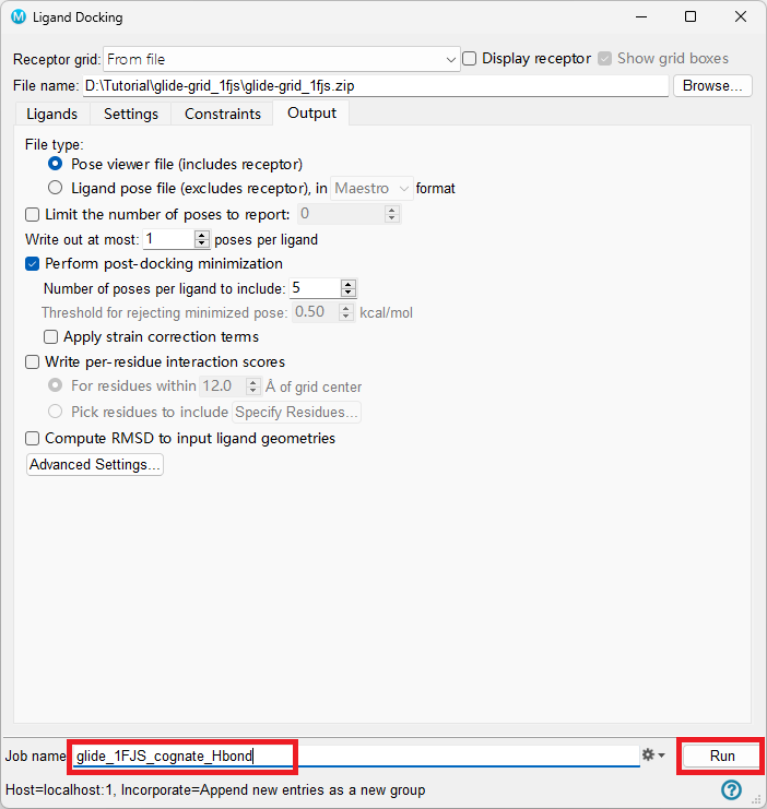
Figure 5-7. The Settings tab of the Ligand Docking panel.

Note

Write per-residue interaction scores option and settings

• Write out per-residue interaction scores for a specified set of residues. The Coulomb, van der Waals, and hydrogen bonding scores, the sum of these three (Eint), and the minimum distances are calculated between the ligand and the specified residues. These values are written as structure-level properties for each ligand to the pose file, as well as to the log file. The residues can be specified by selecting one of the options described below.

• Per-residue interactions can be visualized in the Workspace when viewing poses. See Viewing Poses for more information.

  • For residues within N Å of grid center option and text box Write scores for complete residues that have any atom within the specified distance of the grid center.

13. Click the icon next to the glide-1FJS_cognate_Hbond_pv and select View Poses
14. In the Pose Viewer panel, select Set Up Poses

• The 1fjs_prep_complex entry is fixed in the Workspace, the top 1fjs_prep_lig entry is included, and the Pose Viewer panel appears

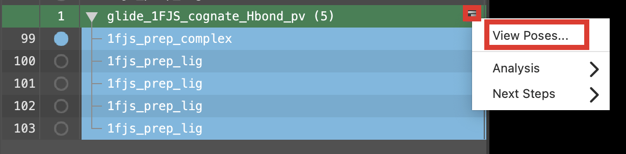
Figure 5-8. View Poses of the cognate ligand. The poses are ranked with the best docking score at the top.

15. Include other ligand results

• H-bonds to ASP 189 are conserved

16. Double-click the In circle next to 1fjs_prep_complex

• The entry is no longer fixed in the Workspace

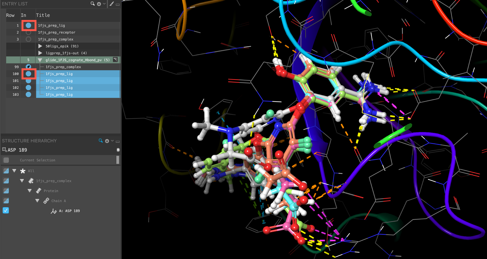
Figure 5-9. Docking result poses shown against the cognate ligand (gray).

Note

To view all docked ligands in their own color, include all ligands to be evaluated and double click the Presets button, or include all ligands and choose Binding Mode Comparison in the Presets menu.

17. Click the cog and choose Show Property

18. Search and add Docking score to the Project Table

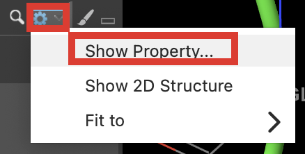
Figure 5-10. Show Property

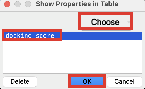
Figure 5-11. Add docking score to the Entry List.

19. Include the top docked pose (the pose with the most negative docking score) and 1fjs_prep_lig to compare the best docked pose to the cognate ligand

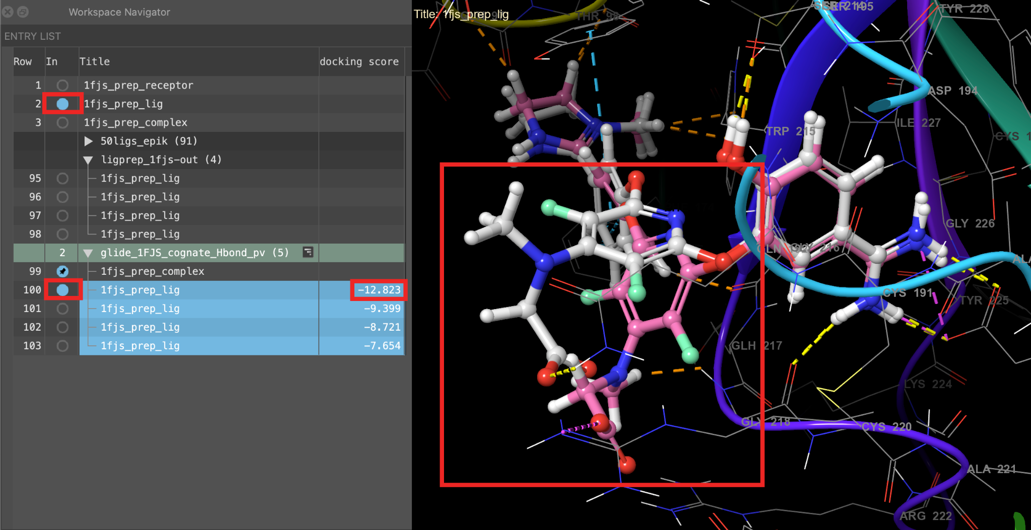
Figure 5-12. An overlay of the best docked pose (pink) with the crystal structure (gray).

Note

Likewise, we can perform virtual screening with above steps.

References

[1] Introduction to Structure Preparation and Visualization (schrodinger.com)

[2] Preparation Workflow Tab (schrodinger.com)

[3] Preparation Workflow Tab (schrodinger.com)

[4] Structure-Based Virtual Screening Using Glide (schrodinger.com)

[5] Receptor Tab (schrodinger.com)