Schrödinger Notes—Field-based QSAR
Declaration
This tutorial is based on the Schrödinger Product Documentation, “Field-based QSAR”1, and created with the Schrödinger Software Release 2023-4.
This note contains only minimal annotations to the original text, along with corrections to formatting errors. It is intended for educational and communicative purposes only, and all rights remain with the original author.
Copying the Field-Based QSAR Exercise Files
Use the following link to download the zip archive that contains the tutorial files: https://content.schrodinger.com/quick_start_guide/current/field_qsar.zip
Unzip the files into your working directory.
Choose File → Change Working Directory in Maestro to set the working directory to where you unzipped the files, if needed.
Adding and Assigning the Ligands for Field-Based QSAR
To set up a QSAR model, you must add ligands and assign them to a training set and a test set. It is always important to have a test set so that you can assess the quality of the model.
- Click the Tasks button and browse to Lead Optimization → 3D Field-Based.
- The Field-Based QSAR panel opens.
- For Add ligands, click From File.
- The Add From File file selector opens.
- Select cdk2_fqsar.maegz and click Open.
- The Choose Activity Property dialog box opens.
Under Choose an activity property, select the pIC50 property.
Click OK.
- The Ligands table in the Field-Based QSAR panel is populated with the 71 ligands. The QSAR Set property is set to training, and the Activity property shows the pIC50 values.
Select rows 55 through 71 in the table (use shift-click).
Control-click the QSAR Set column for one of these rows.
- The value in the column changes to test for all of the selected rows.
When building a model, you must choose which fields to include in the model, and set parameters for building the model. In this exercise, the Gaussian fields will be used.
Building the Field-Based QSAR Models
When building a model, you must choose which fields to include in the model, and set parameters for building the model. In this exercise, the Gaussian fields will be used.
- Click Build.
- The Build Field-Based Model dialog box opens.
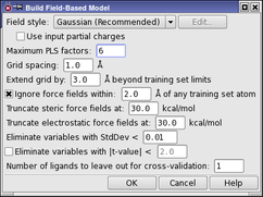
- Set the Field style to Gaussian (Recommended), if it is not already set to this choice.
Force field—Use the force-field electrostatic and steric fields for the model (CoMFA).
Gaussian—Use the five standard Gaussian fields for the model, excluding aromatic ring fields (CoMSIA).
Extended Gaussian—Use all the Gaussian fields for the model, including aromatic ring fields.
Custom—Select the combination of force-field and Gaussian fields to use for the model. To make the selection, click Edit, and select the fields from the list in the Custom Field Style dialog box. In this dialog box you can also import feature definitions for the fields.
- Enter 6 in the Maximum PLS factors text box.
This value should be no more than the number of training set structures divided by 5, otherwise overfitting may occur. A model is built for each number of PLS factors up to this value.
The remaining settings can be left at their default values.
- Click OK.
- The dialog box closes. After a short while, the results columns in the Ligands table is filled in with the predictions for each of the 6 models, for both the training set and the test set, and the QSAR statistics and Field fractions tables are filled in with the statistics for the models.
Examining the Field-Based QSAR Models
After building a set of models, the next task is to determine which of these models to use. For this purpose, both the training set and the test set results should be examined. To avoid choosing an over-fit model, a good rule is to stop increasing the number of PLS factors when no more improvement is obtained in the results.
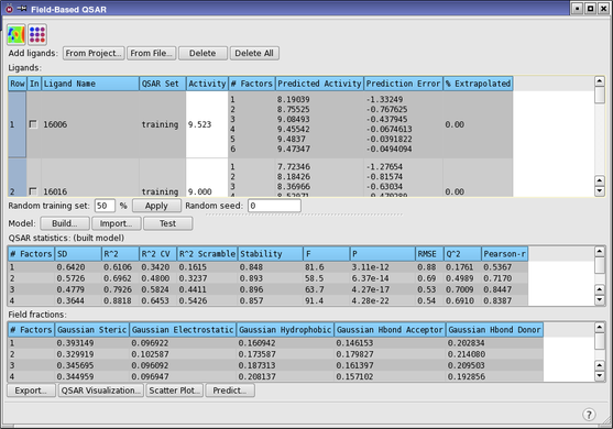
Examine the statistics in the QSAR statistics table.
| Column | Description |
|---|---|
| # Factors | Number of factors in the partial least squares regression model. |
| SD | Standard deviation of the regression. This is the RMS error in the fitted activity values, distributed over n−m−1 degrees of freedom (n ligands, m PLS factors). |
| R^2 | Value of R2 for the regression (the coefficient of determination). A value of 0.80, for example, means that the model accounts for 80% of the variance in the observed activity data. R2 is always between 0 and 1. |
| R^2 CV | Cross-validated R2 value, computed from predictions obtained by a leave-N-out approach. The value of N is specified in the Build Field-Based Model Dialog Box. |
| R^2 Scramble | Average value of R2 from a series of models built using scrambled activities. Measures the degree to which the molecular fields can fit random data. A low value means that the model cannot fit random data, but a high value merely means that the variable set is fairly complete and can fit anything. |
| Stability | Stability of the model predictions to changes in the training set composition. Maximum value is 1. A high value indicates a model that is not sensitive to omissions from the training set. A stability value that is lower than the R2 value is an indication of over-fitting. |
| F | The ratio of the model variance to the observed activity variance. The model variance is distributed over m degrees of freedom and the activity variance is distributed over n−m−1 degrees of freedom (n ligands, m PLS factors). Large values of F indicate a more statistically significant regression. |
| P | The significance level of F when treated as a ratio of Chi-squared distributions. Smaller values indicate a greater degree of confidence. A P value of 0.05 means F is significant at the 95% level. |
| RMSE | Root-mean-square error in the test set predictions. |
| Q^2 | Value of Q2 for the predicted activities. Directly analogous to R-squared, but based on the test set predictions. Q2 can take on negative values if the variance in the errors is larger than the variance in the observed activity values. |
| Pearson-r | Pearson r value for the correlation between the predicted and observed activity for the test set. |
The standard deviation (SD) decreases and the correlation coefficient (R^2) increases as the number of PLS factors increases. R^2 Scramble also increases. This is normal, but does not really tell us much about which model to choose. It only tells us that increasing the number of variables in the fit reduces the error of the fit.
Stability increases to 3 factors, then decreases. The 3-factor model predictions are the least sensitive to the composition of the training set, based on leave-1-out tests. For 4 or more factors, the R^2 value is larger than the stability value, which indicates that over-fitting starts at about 4 factors.
The RMSE decreases from 1 to 3 factors, then doesn’t change much with more factors. Likewise, Q^2 and Pearson-r increase up to 3 factors and don’t change a lot subsequently. As these are test set results, they are a better indicator of the value of adding more factors.
On the basis of these observations, the 3-factor model is probably the best choice, as increasing the number of factors doesn’t improve the test set predictions much, and the models with higher numbers of factors are probably over-fit.
Examining the Training and Test Set Predictions for Field-Based QSAR
Having looked at the overall statistics, we now look at the predictions for both the training set and the test set, using the plotting facility.
- Click Scatter Plot.
- The Phase QSAR - Scatter Plot dialog box opens.
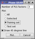
In the Number of PLS factors text box, enter 3.
Select Training set.
Ensure that Draw 45 degree line is selected.
Click Plot.
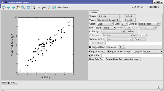
After a short delay, a scatter plot of the training set activities is displayed, labeled plot-1. Nearly all of the points are close to the line, so the training set fit is generally good.
Now plot the test set data.
- Click Scatter Plot (in the Field-Based QSAR panel).
- The Phase QSAR - Scatter Plot dialog box opens again.
Select Test set.
Click Plot.
- A scatter plot of the test set activities is displayed, labeled plot-2.

There are two main outliers, which we will examine.
- Click the In button.

This button allows you to pick points on the plot and have them displayed in the Workspace.
- Pick the two outlying points on the plot, in turn.
- These are for ligands 16047 and 16076. Ligand 16047 has the largest error. There is a similar ligand in the training set, ligand 16058 (row 21) that has a small error.
- In the Field-Based QSAR panel, click the In column in row 21.
- Ligand 16058 is placed in the Workspace.
- Scroll down and control-click the In column in row 68 (ligand 16047)
- Ligand 16047 is also placed in the Workspace, superimposed on ligand 16058. The two ligands are very similar in shape and structure.
- In the Workspace Configuration toolbox, click the Tile button.

The two structures are displayed separately, as shown below (ligand 16058, left, and ligand 16047, right).
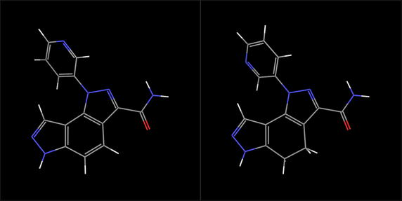
The differences between the two can be seen more easily: the orientation of the pyridyl ring, and the bond order of a carbon-carbon bond in the middle ring of the fused ring system. The first difference would be eliminated if the pyridyl ring were rotated by 180º, which we will do in the next exercise.
- Click Tile again, to exit tile mode.
Field-Based QSAR Visualization
Include either ligand in Field-Based QSAR panel to display in the Workspace.
Click QSAR Visualization in Field-Based QSAR panel to open Field-Based QSAR Visualization Settings panel.
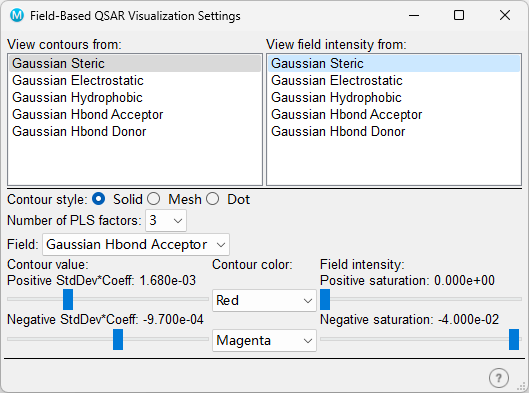
Select one or more fields from "View contours from"list or/and "View field intensity from" list.
Go back to Field-Based QSAR panel, click
 "View
Contours" and
"View
Contours" and  "View Intensities" botton to visualize the
QSAR fields in Workspace.
"View Intensities" botton to visualize the
QSAR fields in Workspace.You can also change the color of Positive/Negative filed in Field-Based QSAR Visualization Settings panel.
A positive region for a Gaussian field means that it is favorable for the field property, and a negative value means that it is unfavorable. For electrostatic fields, a positive region is favorable for positive charges, and a negative region is favorable for negative charges.
Making a Prediction from Field-Based QSAR for a New Ligand
In this exercise, we will modify the structure of one of the outliers from the test set (ligand 16047) and predict its activity. This process illustrates one way to test whether a structural feature is important for activity or not.
- In the Entry List panel, enter 16047 in the filter (search) text box.
- The Entry List panel is docked in the main window by default. If it is not displayed, choose Window → Workspace Navigator.
When you enter the text, only ligand 16047 is listed.
- Click the row for the ligand to select just this ligand.
- The filter doesn’t change the selection of entries, only the entries that are shown. The status report below the list of entries should show Entries: 71 total, 1 selected.
- Right-click in the row and choose Duplicate → In Place.
- The entry for this ligand is duplicated.
Right-click on the duplicated row and choose Move to Row.
Click First, then click Move.
- The duplicated entry becomes row 1. If the duplicate is not included in the Workspace, click the In column in row 1 to place it in the Workspace.
- Right-click the bond between the pyridyl ring and the pyrazole nitrogen, and choose Rotate Dihedral.
- A light blue arrow is displayed, pointing to the pyridyl ring.
- Drag horizontally in the Workspace with the left mouse button to rotate the pyridyl ring by 180°.
- The initial angle (136.2°) and current angle are displayed in the status bar as you drag. The final angle should be close to −43.8°.
- In the Field-Based QSAR panel, click Predict.
- The Choose Entries dialog box opens, so you can choose project entries to predict their activities. By default, only the selected entries are shown, so the ligand you just adjusted should be the only ligand listed.
- Click Choose.
- The dialog box closes, and the prediction is made. The results for all 6 models are added to the Project Table as properties for this ligand.
Press Ctrl+T (⌘T) to open the Project Table panel.
Scroll the table horizontally so that the Activity column is showing.
- The measured activity value is about 5.8.
- Scroll horizontally to view and compare the two sets of predicted activities.
- The first set (Predicted Activityn) is the set for the original structure, and was copied when the structure was duplicated. The second set (predicted activityn) contains the predictions for the modified structure.
The two sets of predictions are almost identical. The model shows no difference resulting from the rotation of this group, and implies that the change in orientation of the pyridyl ring is not relevant to activity.